

Statistical analysis involves the exploration of trends, patterns, and relationships through quantitative data. It serves as a crucial research tool for scientists, governments, businesses, and various organizations.
To draw valid conclusions, careful planning is essential from the inception of the research process. This includes specifying hypotheses and making decisions regarding research design, sample size, and sampling procedures.
After collecting data from the sample, the information can be organized and summarized using descriptive statistics. Subsequently, inferential statistics can be employed to formally test hypotheses and make estimates about the population. Finally, the findings can be interpreted and generalized.
This article serves as an introduction to statistical analysis for students and researchers, guiding them through the steps using two research examples.
The first example delves into a correlational research question, investigating the relationship between parental income and college grade point average (GPA).
The second example explores a potential cause-and-effect relationship, examining whether meditation can enhance exam performance in teenagers.
Read More:
Covariate in Statistics: Examples
How To Calculate the Sample Size for Randomized Controlled Trials (RCT)
What is Primary Data Collection? Types, Advantages, and Disadvantages
How Do You Avoid Common Mistakes in Statistics?
How to build a PLS-SEM model using AMOS?
Understanding Standard Deviation: A Deep Dive into the Key Concepts
Steps of Statistical Analysis Process
Step 1: Develop Your Research Design and Hypotheses
To gather valid data for statistical analysis, it’s crucial to develop hypotheses and outline the research design.
Formulating Statistical Hypotheses
Formulating Statistical Hypotheses Research often aims to explore relationships between variables within a population. The process begins with a prediction, and statistical analysis is employed to test that prediction.
A statistical hypothesis is a formal expression of a prediction about a population. Each research prediction is translated into null and alternative hypotheses, which can be tested using sample data.
The null hypothesis consistently posits no effect or relationship between variables, while the alternative hypothesis presents the research prediction of an effect or relationship.
Example: Hypotheses for Testing a Correlation
- Null hypothesis: There is no relationship between family income and GPA in university students.
- Alternative hypothesis: In university students, there is a positive relationship between family income and GPA.
Example: Hypotheses for Testing an Effect
- Null hypothesis: Teenagers’ math test scores will not be impacted by a 10-minute meditation activity.
- Alternative hypothesis: Teenagers who practice meditation for ten minutes will perform better on math tests.
Developing Research Design
Your research design is the comprehensive strategy for data collection and analysis, shaping the statistical tests applicable to test your hypotheses later.
Begin by determining whether your research will adopt a descriptive, correlational, or experimental design. Experiments exert direct influence on variables, whereas descriptive and correlational studies merely measure variables.
correlational design
In a correlational design, you can investigate relationships between variables (e.g., family income and GPA) without assuming causality, utilizing correlation coefficients and significance tests.
experimental design
In an experimental design, you can evaluate cause-and-effect relationships (e.g., the impact of meditation on test scores) using statistical tests of comparison or regression.
descriptive design
In a descriptive design, you can scrutinize the characteristics of a population or phenomenon (e.g., the prevalence of anxiety in U.K. university students) and draw inferences from sample data using statistical tests.
Your research design will also address whether you will compare participants at the group, individual, or both levels.
between-subjects design
Group-level outcomes of individuals exposed to various treatments (e.g., those who undertook an exercise in meditation vs. those who did not) are compared in a between-subjects design.
within-subjects design
You compare repeated measures from participants participating in all treatments (e.g., scores before and after a meditation exercise) in a within-subjects design.
mixed design
One variable (e.g., pretest and posttest scores from participants who either did or did not undertake a meditation exercise) is manipulated between subjects in a mixed design, while another variable is manipulated within subjects.
Example: Correlational Research Design
In a correlational study, the objective is to explore the relationship between family income and GPA in graduating university students. To gather data, participants will be asked to complete a survey, self-reporting their parents’ incomes and their own GPA.
Unlike experimental designs, there are no distinct dependent or independent variables in this study. The focus is on measuring variables without actively influencing them. The aim is to examine the natural associations between family income and GPA without any experimental interventions.
Example: Experimental Research Design
Imagine designing a within-subjects experiment to investigate whether a 10-minute meditation exercise can enhance math test scores. Your study involves taking repeated measures from a single group of participants.
Here’s the process:
- Obtain baseline test scores from participants.
- Have participants engage in a 10-minute meditation exercise.
- Record participants’ scores from a second math test.
The 10-minute meditation exercise acts as the independent variable in this experiment, and the math test scores obtained both before and after the intervention act as the dependent variable.
Read More:
A Glance At Derivatives & Formulas!
Principal Components Analysis (PCA) using SPSS
What is Multivariate Analysis?
Using Different Statistical Tools: A Guide to Choosing the Right Tool for Data Analysis
Type I vs Type II error in Hypothesis Testing
operationalizing your variables
When devising a research design, it’s crucial to operationalize your variables and determine precisely how you will measure them.
For statistical analysis, the level of measurement of your variables is a key consideration, indicating the nature of the data they encompass:
- Groupings can be nominal or ordinal in categorical data.
- Quantitative data is a representation of amounts that can be on an interval or ratio scale.
Variables may be measured at different levels of precision. For instance, age data can be either quantitative (e.g., 9 years old) or categorical (e.g., young). The numerical coding of a variable (e.g., a rating from 1–5 indicating the level of agreement) does not automatically determine its measurement level.
Choosing the right statistical methods and hypothesis testing requires knowing the measurement level. For example, with quantitative data, you can determine a mean score, but not with categorical data.
In addition to measuring variables of interest, data on relevant participant characteristics is frequently collected in a research study.
Read More:
Measurement of Scale | Examples | PPT
Mixed Method Research: What It Is & Why You Should Use It
Types of Validity in Research | Examples | PPT
Example: nature of variables in Correlational Study
In a correlational study, the nature of the variables determines the test used for a correlation coefficient. When dealing with quantitative data, a parametric correlation test can be used; however, if one of the variables is ordinal, a non-parametric correlation test must be conducted.
| Variable | Data Type |
|---|---|
| Family income | Quantitative (ratio) |
| GPA | Quantitative (interval) |
Example: nature of variables in Experiment
While categorical variables can be used to determine groupings for comparison tests, quantitative age or test score data can be subjected to a number of calculations.
| Variable | Data Type |
|---|---|
| Age | Quantitative (ratio) |
| Gender | Categorical (nominal) |
| Race or ethnicity | Categorical (nominal) |
| Baseline test scores | Quantitative (interval) |
| Final test scores | Quantitative (interval) |
Step 2: Data Collection from a Sample
In most instances, it is impractical or costly to collect data from every individual in the population under study. Consequently, data is often gathered from a sample.
Statistical analysis allows for the extrapolation of findings beyond the sample as long as appropriate sampling procedures are employed. The goal is to have a sample that accurately represents the population.
Two primary approaches are employed in sample selection:
- Probability Sampling: Each member of the population has an equal chance of being chosen through random selection.
- Non-Probability Sampling: Certain members of the population are more likely to be chosen on the basis of convenient or voluntary self-selection criteria.
In theory, for highly generalizable results, probability sampling is preferred. Random selection minimizes various forms of research bias, like sampling bias, ensuring that the sample data is genuinely representative of the population. Parametric tests can then be used for robust statistical inferences.
However, in practice, it’s often challenging to achieve an ideal sample. Non-probability samples are more susceptible to biases like self-selection bias, but they are more accessible for recruitment and data collection. Non-parametric tests are suitable for non-probability samples, although they lead to weaker inferences about the population.
If you wish to employ parametric tests for non-probability samples, you need to argue:
- Your sample is a true representation of the population you aim to generalize your findings to.
- Your sample is devoid of systematic bias.
It is important to understand that applying external validity requires you to limit the generalization of findings to individuals who possess similar characteristics to your sample. For instance, findings from samples that are Western, educated, Industrialized, Rich, and Democratic cannot be generalized to all non-WEIRD populations.
When applying parametric tests to data from non-probability samples, it’s essential to discuss the limitations of generalizing your results in the discussion section.
Read More:
Difference between Descriptive and Inferential Statistics
Friedman Test: Example, and Assumptions
T-test | Example, Formula | When to Use a T-test
Chi-Square Test (Χ²) || Examples, Types, and Assumptions
Develop an Effective Sampling Strategy
Decide how you will recruit participants based on the resources available for your research.
- Will you have the means to advertise your research broadly, even outside of the confines of your university?
- Will you be able to assemble a representative sample of the entire population that is diverse?
- Are you able to follow up with members of groups who are difficult to reach?
Example:
The primary population of interest is male university students in the United States. To gather participants, you utilize social media advertising and target senior-year male university students from a more specific subpopulation—namely, seven universities in the Boston area. In this scenario, participants willingly volunteer for the survey, indicating that this is a non-probability sample.
Example:
The focus is on the population of university students in your city. To recruit participants, you reach out to three private schools and seven public schools across different districts within the city, intending to conduct your experiment with bachelor’s students. The participants in this case are self-selected through their universities. Despite the use of a non-probability sample, efforts are made to ensure a diverse and representative sample.
Determine the Appropriate Sample Size
Before initiating the participant recruitment process, establish the sample size for your study. This can be accomplished by reviewing existing studies in your field or utilizing statistical methods. It’s crucial to avoid a sample that is too small, as it may not accurately represent the population, while an excessively large sample can incur unnecessary costs.
Several online sample size calculators are available, each using different formulas depending on factors such as the presence of subgroups or the desired rigor of the study (e.g., in clinical research). A general guideline is to have a minimum of 30 units per subgroup. To utilize these calculators effectively, you need to comprehend and input key components:
- Significance level (alpha): This is the risk of incorrectly rejecting a true null hypothesis, typically set at 5%.
- Population standard deviation: This is an estimate of the population parameter derived from a previous study or a pilot study conducted for your research.
- Expected effect size: This is a standardized measure of the anticipated magnitude of the study’s results, often based on similar studies.
- Statistical power: This is the likelihood that your study will detect an effect of a certain size if it exists, usually set at 80% or higher.
Step 3: Summarize Your Data Using Descriptive Statistics
After gathering all your data, the next step is to examine and summarize them using descriptive statistics.
Analyzing Data
- Organize Data: Create frequency distribution tables for each variable.
- Visual Representation: Use bar charts to illustrate the distribution of responses for a key variable.
- Explore Relationships: Utilize scatter plots to visualize the relationship between two variables.
By presenting your data in tables and graphs, you can evaluate whether the data exhibit a skewed or normal distribution and identify any outliers or missing data.
A normal distribution indicates that the data are symmetrically distributed around a central point, with the majority of values clustered there and tapering off towards the tail ends.
In contrast, a skewed distribution is asymmetrical and exhibits more values on one end than the other. Understanding the distribution’s shape is crucial because certain descriptive statistics are more suitable for skewed distributions.
The presence of extreme outliers can also distort statistics, necessitating a systematic approach to handling such values.
Determine Central Tendency Measures
Measures of central tendency indicate where the majority of values in a data set are concentrated.
The three primary measures are:
- Mode: The most frequent response or value in the data set.
- Median: The middle value when the data set is ordered from low to high.
- Mean: The sum of all values divided by the number of values.
However, the appropriateness of these measures depends on the distribution’s shape and the level of measurement. For instance, demographic characteristics may be described using the mode or proportions, while variables like reaction time may lack a mode.
Measures of Variability
Measures of variability convey how dispersed the values in a data set are. Four main measures are commonly reported:
- Range: The difference between the highest and lowest values in the data set.
- Interquartile Range: The range of the middle half of the data set.
- Standard Deviation: The average distance between each value in the data set and the mean.
- Variance: The square of the standard deviation.
Once again, the choice of variability statistics should be guided by the distribution’s shape and the level of measurement. The interquartile range is preferable for skewed distributions, while standard deviation and variance offer optimal information for normal distributions.
Example: Correlational Study
Following the collection of data from 567 students, descriptive statistics for annual family income and GPA are tabulated.
It is crucial to verify whether there is a broad range of data points. Insufficient variation in data points may result in skewness toward specific groups (e.g., high academic achievers), limiting the generalizability of inferences about a relationship.
| Parental Income (USD) | GPA |
|---|---|
| Mean | 62,100 |
| Standard Deviation | 15,000 |
| Variance | 225,000,000 |
| Range | 8,000–378,000 |
| N | 653 |
Next, the computation of a correlation coefficient and the performance of a statistical test will provide insights into the significance of the relationship between the variables in the population.
Example: Experiment
Following the collection of pretest and posttest data from 30 students across the city, descriptive statistics are calculated. Given the normal distribution of data on an interval scale, the mean, standard deviation, variance, and range are tabulated.
It is crucial to examine whether the units of descriptive statistics are comparable for pretest and posttest scores using the table. Specifically, one should assess whether the variance levels are similar across the groups and identify any extreme values. If extreme outliers are present, they may need identification and removal from the dataset, or data transformation may be required before conducting a statistical test.
| Pretest Scores | Posttest Scores |
|---|---|
| Mean | 68.44 |
| Standard Deviation | 9.43 |
| Variance | 88.96 |
| Range | 36.25 |
| N | 30 |
This table shows that following the meditation exercise, the mean score increased, and the variances of the two scores are similar. To find out if this increase in test scores is statistically significant throughout the population, a statistical test must be performed.
Step 4: Use Inferential Statistics to Test Hypotheses or Make Estimates
A numerical description of a sample is termed a statistic, while a number characterizing a population is referred to as a parameter. Inferential statistics enable drawing conclusions about population parameters based on sample statistics.
Researchers commonly employ two primary methods concurrently for statistical inferences:
- Estimation: This involves calculating population parameters based on sample statistics.
- Hypothesis Testing: It is a formal process for assessing research predictions about the population using samples.
Estimation
There are two types of estimates for population parameters derived from sample statistics:
- Point Estimate: A single value representing the best guess of the exact parameter.
- Interval Estimate: A range of values representing the best guess of the parameter’s location.
In cases where the goal is to infer and report population characteristics from sample data, utilizing both point and interval estimates is advisable.
A sample statistic can serve as a point estimate for the population parameter when dealing with a representative sample. For instance, in a broad public opinion poll, the proportion of a sample supporting the current government is considered the population proportion of government supporters.
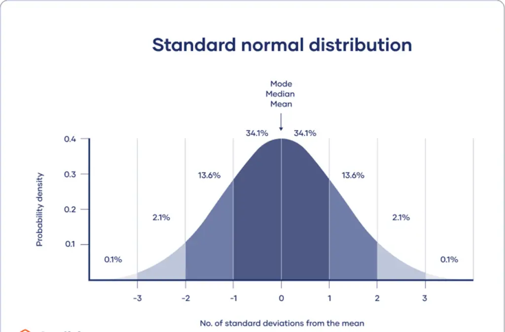
As estimation inherently involves error, providing a confidence interval as an interval estimate is essential to illustrate the variability around a point estimate. A confidence interval utilizes the standard error and the z-score from the standard normal distribution to indicate the range where the population parameter is likely to be found most of the time.
Hypothesis Testing
Testing hypotheses includes using data from a sample to assess hypotheses regarding the relationships between variables in the population. The null hypothesis is first assumed to be true for the population, and statistical tests are then used to see if the null hypothesis can be rejected.
Statistical tests ascertain where your sample data would fall on an expected distribution of sample data under the assumption that the null hypothesis is true. These tests yield two primary outcomes:
- Test Statistic: Indicates the extent to which your data deviates from the null hypothesis.
- p-value: Represents the likelihood of obtaining your results if the null hypothesis is indeed true in the population.
Statistical tests fall into three main categories:
- Regression Tests: Evaluate cause-and-effect relationships between variables.
- Comparison Tests: Assess group differences in outcomes.
- Correlation Tests: Examine relationships between variables without assuming causation.
A number of factors, such as the research questions, sampling method, research design, and data characteristics, influence the choice of statistical test.
Parametric Tests
Parametric tests enable robust inferences about the population based on sample data. However, certain assumptions must be met, and only specific types of variables can be used. If these assumptions are violated, appropriate data transformations or alternative non-parametric tests should be considered.
- Regression: Calculates the degree to which changes in one or more predictor variables affect the corresponding outcome variable.
- Simple Linear Regression: Involves one predictor variable and one outcome variable.
- Multiple Linear Regression: Incorporates two or more predictor variables and one outcome variable.
- Comparison Tests: Typically compare means of groups.
- t-test: Applicable for 1 or 2 groups with a small sample size (30 or less).
- z-test: Suitable for 1 or 2 groups with a large sample size.
- ANOVA: Used when comparing means across 3 or more groups.
The z and t tests come with various subtypes based on the number and types of samples, as well as the hypotheses being tested:
- One-Sample Test: Applied when you have only one sample that you want to compare to a population mean.
- Dependent (Paired) Samples Test: Utilized for paired measurements in a within-subjects design.
- Independent (Unpaired) Samples Test: Employed when dealing with completely separate measurements from two unmatched groups in a between-subjects design.
- One-Tailed Test: Preferable if you expect a difference between groups in a specific direction.
- Two-Tailed Test: Suitable when you don’t have expectations for the direction of a difference between groups.
For parametric correlation testing, Pearson’s r is the primary tool. This correlation coefficient (r) gauges the strength of a linear relationship between two quantitative variables.
To assess whether the correlation in the sample holds significance in the population, a significance test of the correlation coefficient is conducted, usually using a t test, to obtain a p-value. This test leverages the sample size to determine how much the correlation coefficient deviates from zero in the population.
Example: Significance Test with Correlation Coefficient:
In investigating the relationship between family income and GPA, Pearson’s r is employed to quantify the strength of the linear correlation within the sample. The calculated Pearson’s r value of 0.12 indicates a small correlation observed in the sample.
While Pearson’s r serves as a test statistic, it alone does not provide insights into the significance of the correlation in the broader population. To ascertain whether this sample correlation is substantial enough to reflect a correlation in the population, a t-test is conducted. In this scenario, anticipating a positive correlation between parental income and GPA, a one-sample, one-tailed t-test is utilized. The results of the t-test are as follows:
- t Value: 3.08
- p Value: 0.001
These outcomes from the statistical test offer insights into the significance of the correlation, helping determine if the observed correlation in the sample holds importance in the broader population.
Example: Experimental Research Using Paired T-Tests:
In the context of a within-subjects experiment design, where both pretest and posttest measurements originate from the same group, a dependent (paired) t-test is employed. Given the anticipation of a change in a specific direction (an enhancement in test scores), a one-tailed test is deemed necessary.
For instance, let’s consider a study evaluating the impact of a meditation exercise on math test scores. Using a dependent-samples, one-tailed t-test, the following results are obtained:
- t Value (Test Statistic): 3.00
- p Value: 0.0028
These outcomes from the statistical test help determine whether the meditation exercise had a statistically significant effect on improving math test scores.
Step 5: Interpretation of the Results
The last step of statistical analysis involves the interpretation of your findings.
Statistically significant
In hypothesis testing, statistical significance stands as the principal criterion for drawing conclusions. The assessment involves comparing the obtained p value with a predetermined significance level, typically set at 0.05. This evaluation determines whether your results hold statistical significance or are deemed non-significant.
Results are deemed statistically significant when the likelihood of their occurrence due to chance alone is exceptionally low. Such outcomes suggest a minimal probability of the null hypothesis being true in the broader population, reinforcing the credibility of the observed results.
Example: Interpret Your Correlational Study Results
Upon comparing the obtained p value of 0.001 with the significance threshold set at 0.05, it is evident that the p value falls below this threshold. Consequently, you can reject the null hypothesis, signifying a statistically significant correlation between parental income and GPA in male college students.
It is essential to acknowledge that correlation does not inherently imply causation. Complex variables like GPA are often influenced by numerous underlying factors. A correlation between two variables may be due to a third variable impacting both or indirect connections between the two variables.
Additionally, it’s crucial to recognize that a large sample size can strongly influence the statistical significance of a correlation coefficient, potentially making even small correlations appear significant.
Example: interpret your experiment’s results
Upon scrutinizing the obtained p value of 0.0027 and comparing it to the predetermined significance threshold of 0.05, you discover that the p value is lower. Consequently, you opt to reject the null hypothesis, establishing your results as statistically significant.
This implies that, in your interpretation, the observed elevation in test scores is attributed to the meditation intervention rather than random factors.
Effect Size
While statistical significance provides information about the likelihood of chance influencing your results, it doesn’t inherently convey the practical importance or clinical relevance of your findings.
On the other hand, the effect size shows how useful your conclusions are in real-world situations. For a comprehensive understanding of your findings, it’s critical to include effect sizes in addition to your inferential statistics. In an APA style paper, you should additionally include interval estimates of the effect sizes.
Example: effect size of the correlation coefficient
When evaluating the effect size of the correlation coefficient, you reference Cohen’s effect size criteria with your Pearson’s r value. Falling between 0.1 and 0.3, your discovery of a correlation between family income and GPA indicates a very small effect, suggesting limited practical significance.
Example: Effect Size of the Experimental Research
In assessing the impact of the meditation exercise on test scores, you compute Cohen’s d, revealing a value of 0.72. This denotes a medium to high level of practical significance, indicating a substantial difference between pretest and posttest scores attributable to the meditation intervention.
Type I and Type II errors
In research conclusions, mistakes can occur in the form of Type I and Type II errors. A Type I error involves rejecting the null hypothesis when it is, in fact, true, while a Type II error occurs when the null hypothesis is not rejected when it is false.
Making sure there is high power and choosing the ideal significance level are crucial steps in reducing the possibility of these errors. But there is a trade-off between the two types of errors, so one needs to consider them carefully.
Bayesian Statistics versus Frequentist statistics
Frequentist statistics has traditionally focused on testing the significance of the null hypothesis and started with the assumption that the null hypothesis is true. In contrast, Bayesian statistics have become more prevalent as an alternative approach.
In Bayesian statistics, previous research is used to continuously update hypotheses based on expectations and observations.
In Bayesian statistics, the Bayes factor is a fundamental concept that compares the relative strength of evidence supporting the alternative hypothesis against the null hypothesis without necessarily concluding that the null hypothesis should be rejected.